Project 1: Boston Housing Prices Dataset

This project is part of Udacity’s Machine Learning Nanodegree. My solutions to the code is located at https://github.com/Edderic/udacity-machine-learning-nanodegree/blob/master/p1-boston-housing-prices/boston_housing_students.py

Task

You want to be the best real estate agent out there. In order to compete with other agents in your area, you decide to use machine learning. You are going to use various statistical analysis tools to build the best model to predict the value of a given house. Your task is to find the best price your client can sell their house at. The best guess from a model is one that best generalizes the data.

I: Statistical Analysis and Data Exploration

There are \(506\) data points. The mean housing price is \($22,532.81\). The median value is \($21,200.00\). The standard deviation is \($9,197.10\). The minimum median value (MEDV) is \($5,000.00\), while the max MEDV is \($50,000.00\)

A comparison of features as they relate to the median value are as follows:

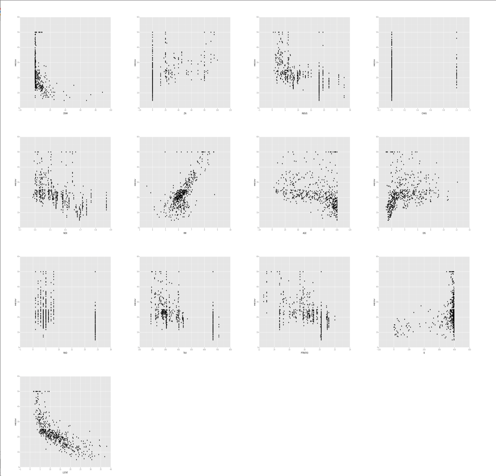
Judging from a quick glance of the graphs, I would say that the best features to predict median value are crime rate (CRIM), number of rooms (RM), and lower status (LSTAT). Lower crime rates, higher number of rooms, and higher status of people living in an area seem to be strongly correlated with higher median values. The rest of the features seem to have predictive power as well. For example, increases in nitrous oxide levels (NOX) seem to be negatively correlated with MEDV. However, NOX, along with other features not previously mentioned, seem to output a bigger range of values given a certain input (i.e. less strongly correlated).

II: Evaluating Model Performance

Which measure of model performance is best to use for regression and predicting Boston housing data? Why is this measurement most appropriate? Why might the other measurements not be appropriate here?

We use the Mean Squared Error (MSE) as a performance metric. The main reason we are using it is because of implementation necessities. The regressor of choice for this project is Scikit’s DecisionTree Regressor, which only works with MSE (and does not work with other metrics like Mean Absolute Error (MAE)) See ‘criterion’ at http://scikit-learn.org/stable/modules/generated/sklearn.tree.DecisionTreeRegressor.html. The regressor might be exploiting the fact that MSE is differentiable (i.e. the local minima of the error function can be found by finding the point where the derivative of the MSE is zero and the second derivative is positive).

Why is it important to split the data into training and testing data? What happens if you do not do this?

It is important to split the data to training and test sets because it gives us a way to somehow measure how our model is going to perform with future (unknown) data. More training data is generally a good thing. This means that we have more data to learn from. However, if we use so much of the data for training purposes and not have enough (or even any) for the test set, we increase the chances of possibly overfit the data set, not generalize well to future data, resulting in poor predictive performance. Test sets are a proxy for how well our model will perform with future data.

Which cross validation technique do you think is most appropriate and why?

If training and testing time are of utmost importance, then the simple train_test_split procedure might be sufficient. However, in order to really improve the performance of the model, without worrying about having the best training and run time, k-fold cross validation technique is most-appropriate. It lets us reappropriate test data for training data, and vice versa, and gives us an averaged score, so it’s accuracy should be more robust than the former. The specific variations of k-fold cross validation, such as Stratified k-fold and Label k-fold do not apply to our problem because they are meant for classification problems, not regression problems. See the following for an example: http://scikit-learn.org/stable/modules/generated/sklearn.cross_validation.StratifiedKFold.html#sklearn.cross_validation.StratifiedKFold

What does grid search do and why might you want to use it?

There are usually a lot of parameters that we can tweak to optimize the performance of our model. Grid search lets us specify those parameters that we want to tweak, the ranges that should be explored for each parameter, and the scoring function that we want to optimize. It then iteratively searches the combinations of those parameters and gives us the values of the parameters that optimize the scoring function. This is a methodical, automatic way to find the best values for the parameters that could save Machine Learning practitioners time. It is especially helpful when there are so many parameters to tweak. Learn more about GridSearch here: http://scikit-learn.org/stable/modules/generated/sklearn.grid_search.GridSearchCV.html

III: Analyzing Model Performance

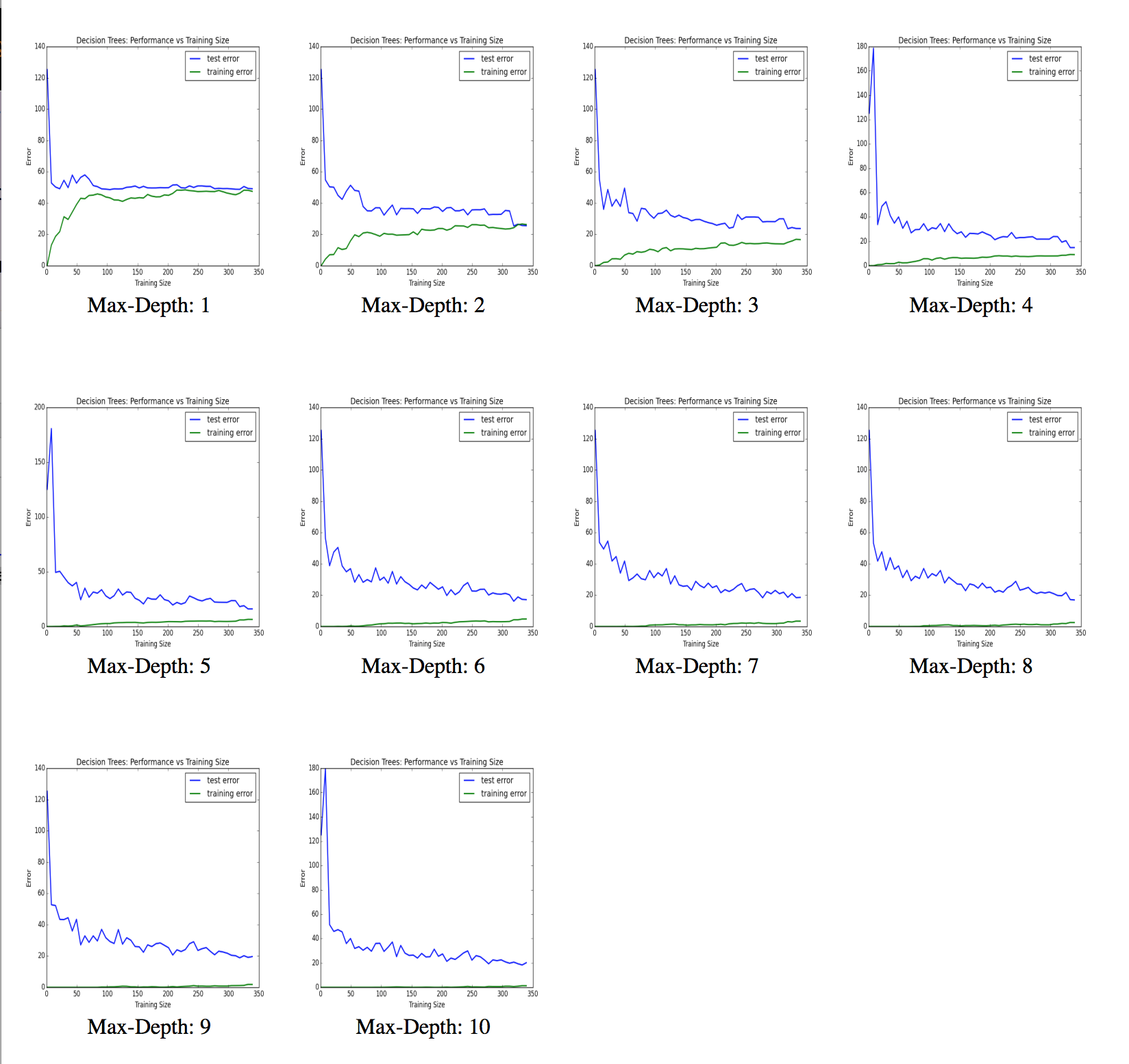
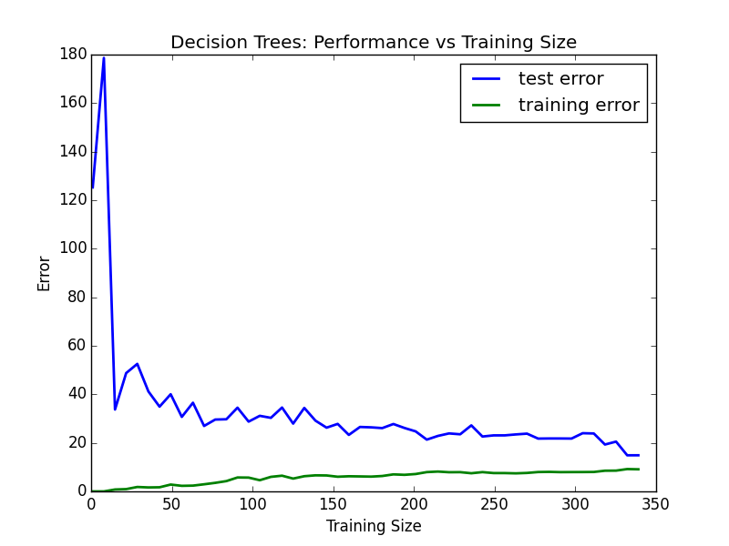
Look at all learning curve graphs provided. What is the general trend of training and testing error as training size increases?

The general trend of training and testing error as training size increases are as follows. The model, in general, gets better and better with training data. When the training size is small, the training errors start out being tiny. This is because the model has “memorized” the (small) training set and does well with the (small) training set. It however, does very poorly on the test set because it hasn’t been trained with enough examples. Once the training size increases, the training error starts to increase by some amount, depending on whether the model is overfitting or underfitting (if underfitting, the increase in training error is high. If overfitting, the increase in training error is low). Because it was given more training examples, it performs better in predicting unseen (test) data. Hence, we see the test error dip down. Given even more data, both training and test errors seem to be following a horizontal asymptote.

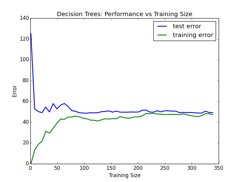
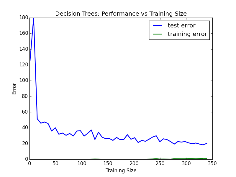
Look at the learning curves for the decision tree regressor with max depth 1 and 10 (first and last learning curve graphs). When the model is fully trained does it suffer from either high bias/underfitting or high variance/overfitting?

When max depth was \(1\), the model was suffering from high bias. The model was performing poorly not only on the test set, but also on the training set. This means that no matter how much data we give it, it does not capture the patterns in the data that help us improve predictive performance.

On the other hand, when the max depth was \(10\), the model was suffering from overfitting. In this case, the training error was virtually nil. However, the test error was still significant. The model, at this point, has “memorized” the training set such that the training error is low, but cannot generalize well enough to do well with unseen data.

Look at the model complexity graph. How do the training and test error relate to increasing model complexity? Based on this relationship, which model (max depth) best generalizes the dataset and why?

As a model starts from being simple to becoming more complex, both the training and test error improves. However, at a certain point, the test error starts to increase again, while the training error keeps decreasing. This is a sign that we have gotten past the sweet spot, and are starting to overfit. It looks like max depth of 4 best generalizes the dataset for these reasons. At max depth of \(4\), the mean squared error (MSE) is hovering around \(\approx 18\).

IV: Model Prediction

For a house with the features:

GridSearch with the parameters below gives us a prediction of \($21,629.74\). This is only about \($400\) more than the median, and about \($900\) less than the mean.

Here are the actual parameters that gave us the prediction:

DecisionTreeRegressor(criterion='mse', max_depth=4, max_features=None,
           max_leaf_nodes=None, min_samples_leaf=1, min_samples_split=2,
           min_weight_fraction_leaf=0.0, random_state=None,
           splitter='best')

The suggested price is within \(1\)-standard deviation of the mean, so the price definitely does not seem like it might be an outlier that might warrant stringent inquiry. Thus, given the features of the house, relative to other houses, \(\approx $21,600.00\) is a good, fair price to sell.