Udacity MLND P4: Train a Smartcab

Code

Code can be found here

Tasks

Implement a basic driving agent

Implement the basic driving agent, which processes the following inputs at each time step:

Next waypoint location, relative to its current location and heading, Intersection state (traffic light and presence of cars), and, Current deadline value (time steps remaining), And produces some random move/action (None, ‘forward’, ‘left’, ‘right’). Don’t try to implement the correct strategy! That’s exactly what your agent is supposed to learn.

Run this agent within the simulation environment with enforce_deadline set to False (see run function in agent.py), and observe how it performs. In this mode, the agent is given unlimited time to reach the destination. The current state, action taken by your agent and reward/penalty earned are shown in the simulator.

In your report, mention what you see in the agent’s behavior. Does it eventually make it to the target location?

The agent is randomly picking actions, no matter what the condition of the environment. It does not care whether or not there is an oncoming vehicle, nor does it care about vehicles on its left nor right. It also seems to disregard the traffic light.

It seems to reward the following:

Going right when traffic light is red:

LearningAgent.update(): deadline = 20,
 inputs = {'light': 'red',
 'oncoming': None,
 'right': None,
 'left': None},
 action = right,
 reward = 2

LearningAgent.update(): deadline = 14,
 inputs = {'light': 'red',
 'oncoming': None,
 'right': None,
 'left': None},
 action = right,
 reward = 2

LearningAgent.update(): deadline = 13,
 inputs = {'light': 'red',
 'oncoming': None,
 'right': None,
 'left': None},
 action = right,
 reward = 2

LearningAgent.update(): deadline = 12,
 inputs = {'light': 'red',
 'oncoming': None,
 'right': None,
 'left': None},
 action = right,
 reward = 0.5

LearningAgent.update(): deadline = 11,
 inputs = {'light': 'red',
 'oncoming': None,
 'right': None,
 'left': None},
 action = right,
 reward = 2

LearningAgent.update(): deadline = 8,
 inputs = {'light': 'red',
 'oncoming': None,
 'right': None,
 'left': None},
 action = right,
 reward = 0.5

Going forward when traffic light is green:

LearningAgent.update(): deadline = 19,
 inputs = {'light': 'green',
 'oncoming': None,
 'right': None,
 'left': None},
 action = forward,
 reward = 2

LearningAgent.update(): deadline = 16,
 inputs = {'light': 'green',
 'oncoming': None,
 'right': None,
 'left': None},
 action = forward,
 reward = 0.5

Going forward when traffic light is green and car in the right is trying to move forward:

LearningAgent.update(): deadline = 10,
 inputs = {'light': 'green',
 'oncoming': None,
 'right': 'forward',
 'left': None},
 action = forward,
 reward = 0.5

Going right when traffic light is green:

LearningAgent.update(): deadline = 11,
 inputs = {'light': 'green',
 'oncoming': None,
 'right': None,
 'left': None},
 action = right,
 reward = 2

LearningAgent.update(): deadline = 6,
 inputs = {'light': 'green',
 'oncoming': None,
 'right': None,
 'left': None},
 action = right,
 reward = 0.5

Staying at the same location when deadline is red:

LearningAgent.update(): deadline = 17,
 inputs = {'light': 'red',
 'oncoming': None,
 'right': None,
 'left': None},
 action = None,
 reward = 1

Staying at the same location when stoplight is green:

LearningAgent.update(): deadline = 7,
 inputs = {'light': 'green',
 'oncoming': None,
 'right': None,
 'left': None},
 action = None,
 reward = 1

LearningAgent.update(): deadline = 5,
 inputs = {'light': 'green',
 'oncoming': None,
 'right': None,
 'left': None},
 action = None,
 reward = 1

It penalizes the following:

Going forward when the traffic light is red:

LearningAgent.update(): deadline = 18,
 inputs = {'light': 'red',
 'oncoming': None,
 'right': None,
 'left': None},
 action = forward,
 reward = -1

LearningAgent.update(): deadline = 15,
 inputs = {'light': 'red',
 'oncoming': None,
 'right': None,
 'left': None},
 action = forward,
 reward = -1

Going left when the traffic light is red:

LearningAgent.update(): deadline = 9,
 inputs = {'light': 'red',
 'oncoming': None,
 'right': None,
 'left': None},
 action = left,
 reward = -1

Interesting to note that environment seems to prevent the car from moving forward.

It does eventually make it to the target location, but only through many iterations, and it seems to take so long that it is way past the deadline.

Identify and update state

Identify a set of states that you think are appropriate for modeling the driving agent. The main source of state variables are current inputs, but not all of them may be worth representing. Also, you can choose to explicitly define states, or use some combination (vector) of inputs as an implicit state.

At each time step, process the inputs and update the current state. Run it again (and as often as you need) to observe how the reported state changes through the run.

Justify why you picked these set of states, and how they model the agent and its environment.

I made a decision tree that seems to capture the reward system above:

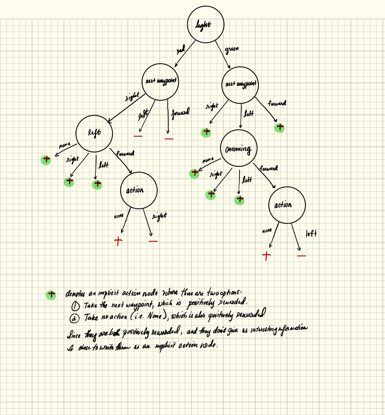
Decision tree that seems to classify correctly when actions should be rewarded or punished. — Smartcab decision tree

One might notice that in the decision tree above, I do not consider the situation where the learning agent decided to turn right when the car is in an intersection where light is red and an oncoming car is turning left. This is because the environment seems to reward such behavior, as seen below:

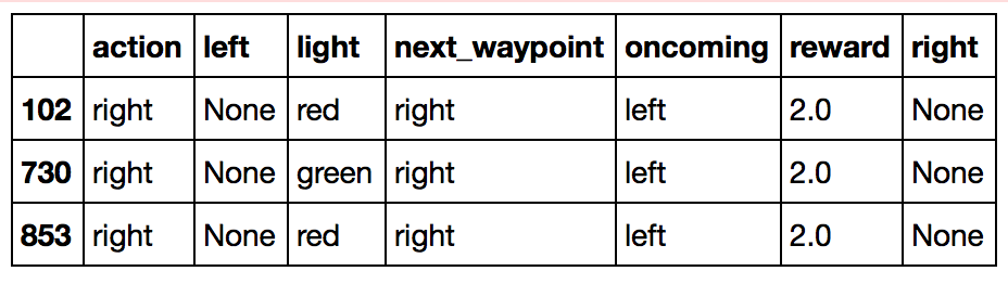
Intersection has a red light. Learning agent wants takes a right, but the oncoming traffic wants to turn left. — Getting positively rewarded for not following part of the U.S. right-of-way

Here are the U.S. right-of-way rules:

When light is green, the learning agent definitely has the right of way when taking the action of moving forward or turning right. The only exception to this is when the learning agent wants to turn left, but there is an oncoming car that is moving forward. In this case, the other car has the right of way. But if there is no car oncoming, the learning agent may turn left.
When light is red, the learning agent may not take the action of turning left or move forward. It could turn right, but only when there is no car on the left, or if there is a car on the left but it is not moving forward.

Thus, it makes sense to fold light, action, and oncoming into one state. It also made sense to consider the next_waypoint because its existence helps guide the agent to bigger rewards (i.e. following the next waypoint when also following the U.S. right-of-way rules results in bigger rewards than just following the U.S. right-of-way rules but meandering aimlessly).

Therefore, the final states to consider are the following.

Light: red or green.
Oncoming: forward, left, or right, or None.
Left: forward, left, or right, or None.
Action: Take the next waypoint, or None.
Next waypoint: forward, left, or right.

Removing any of the first four would seriously impair the learning agent’s ability to learn the right of way, and therefore, would endanger passengers lives. On the other hand, keeping the first four intact, but removing the next waypoint would impair the learning agent from learning the optimal policy; it would be a lot safer – the learning agent would get to learn the right of way, but it might not meet the deadline as it would likely meander around aimlessly.

Thus it is not necessary to add the fold the following state into the table:

Right: forward, left, or right, or None.

Knowing whether a car on the right of the intersection is unnecessary for the q-table. We could still choose to fold it in as part of each state in the table, but that would expand the state space by a lot.

With the $5$ folded states described above, our state-space in the q-table is the following size:

$\begin{align} 2*4*4*2*3 = 192 \end{align}$

By adding right as part of the state, we would still be able to learn the right-of-way, but it would probably take a much longer time to do so, because our state-space would increase to the following:

$\begin{align} 192 * 4 = 768 \end{align}$

Thus, it is important to only consider folding states that are actually relevant to the problem at hand to satisfy the following conditions: 1) that the learning agent learns the right-of-way rules, 2) that it does so in less steps than more (i.e. more efficient).

Originally, I was also considering the deadline to fold into each state of the q-table, but I thought it was unnecessary, as the learning agent seems to learn the right-of-way rules under $100$ trials, and consistently is able to get to the destination safely and on time, maximizing the rewards it got by following the next_waypoint when appropriate. Thus, I did not use deadline at all.

Implement Q-Learning

Implement the Q-Learning algorithm by initializing and updating a table/mapping of Q-values at each time step. Now, instead of randomly selecting an action, pick the best action available from the current state based on Q-values, and return that.

Each action generates a corresponding numeric reward or penalty (which may be zero). Your agent should take this into account when updating Q-values. Run it again, and observe the behavior.

What changes do you notice in the agent’s behavior?

The Learning Agent gets to the destination much faster. In the earlier trials, the agent accumulates both positive and negative rewards (i.e. exploration). In the later trials, the learning agent tends to accumulate only positive rewards (i.e. exploitation).

It seems though, that it learns quickly. In the first $5$ trials, it received some form of punishment (i.e. negative reward), but the next 5 trials, it did not receive punishment at all.

Trial #	received punishment
0	TRUE
1	TRUE
2	FALSE
3	TRUE
4	FALSE
5	FALSE
6	FALSE
7	FALSE
8	FALSE
9	FALSE

Whether or not learning agent has received punishment over first ten trials

Here was the mistake for trial $0$. The Learning Agent learned to not go forward when light is red:

LearningAgent.update(): deadline = 39,
 inputs = {'light': 'red',
 'oncoming': None,
 'right': None,
 'left': None},
 action = forward,
 reward = -1,
 next_waypoint = forward

Here was the mistake for trial $1$, which is similar to the mistake during trial $0$, different only in that there was an oncoming car moving to the left. This makes sense because the two states are different. The Learning Agent learned to not go forward when light is red and when there’s an oncoming car going to oncoming car’s left:

LearningAgent.update(): deadline = 28,
 inputs = {'light': 'red',
 'oncoming': 'left',
 'right': None,
 'left': None},
 action = forward,
 reward = -1,
 next_waypoint = forward

Trial $3$ had a mistake the same as trial $0$:

LearningAgent.update(): deadline = 39,
 inputs = {'light': 'red',
 'oncoming': None,
 'right': None,
 'left': None},
 action = forward,
 reward = -1,
 next_waypoint = forward

Then for a while, it seems to be taking correct actions (trials $4$-$9$). However, this does not mean that the learning agent is already perfect after only 5 trials. It still took incorrect actions intermittently, which are harder-to-catch because they involve cars being present in the learning agent’s view.

Later errors, such as ones from trial $20$, are exemplary of cases where the learning agent is learning to deal with driving rules when other cars are visible:

LearningAgent.update(): deadline = 32,
 inputs = {'light': 'red',
 'oncoming': 'forward',
 'right': None,
 'left': None},
 action = forward,
 reward = -1,
 next_waypoint = forward

LearningAgent.update(): deadline = 31,
 inputs = {'light': 'red',
 'oncoming': 'forward',
 'right': None,
 'left': 'right'},
 action = forward,
 reward = -1,
 next_waypoint = forward

Looking at the tail of the the 100 iterations, we could see that the driving is much improved. It did not get any sort of punishments in the last ten trials:

Trial #	received punishment
90	FALSE
91	FALSE
92	FALSE
93	FALSE
94	FALSE
95	FALSE
96	FALSE
97	FALSE
98	FALSE
99	FALSE

Learning agent's actions in the last ten trials were all correct.

Enhance the driving agent

Apply the reinforcement learning techniques you have learnt, and tweak the parameters (e.g. learning rate, discount factor, action selection method, etc.), to improve the performance of your agent. Your goal is to get it to a point so that within $100$ trials, the agent is able to learn a feasible policy - i.e. reach the destination within the allotted time, with net reward remaining positive.

Report what changes you made to your basic implementation of Q-Learning to achieve the final version of the agent. How well does it perform?

I think the action selection method is quite optimal already in my “basic” implementation of Q-Learning. At any point in time, I made the learning agent only choose between two actions: either choose the next waypoint as the action, or stay in the same intersection. The benefit of this is that there is less space for the learning agent to “explore.” My a priori knowledge of the reward system helped me limit the actions to choices that are generally good choices. Taking the action of going to the next waypoint brings us closer the destination, but risking violating traffic laws. On the other hand, doing nothing does not get us a step closer to reaching the destination, but may prevent violation of traffic laws (and be less of a safety risk). Thus in optimizing my implementation, I chose to fiddle with the learning rate and the discount factor instead.

First, to measure success when comparing different parameters, I thought that looking into $average\ reward\ /\ total\ moves$ might be a good metric to use. For example, let’s assume that there exists two sets of $100$ trials $A$ & $B$. If both sets have the same number of moves, and if the ratio is higher for $A$, than $B$, then $A$ must be incurring more rewards than $B$. Likewise, if $A$ & $B$ got the same reward sum but if $B$ took more moves, then $A$ is more efficient than $B$. This metric is also great because when the learning agent makes mistakes, the environment prevents it from taking a step, which means that the number of actions it takes increases without actually getting closer to the goal. Thus, when it makes a lot of mistakes, the $average\ reward\ /\ total\ moves$ ratio (RPM) will be lower than when it does not make a lot of mistakes, assuming everything else equal.

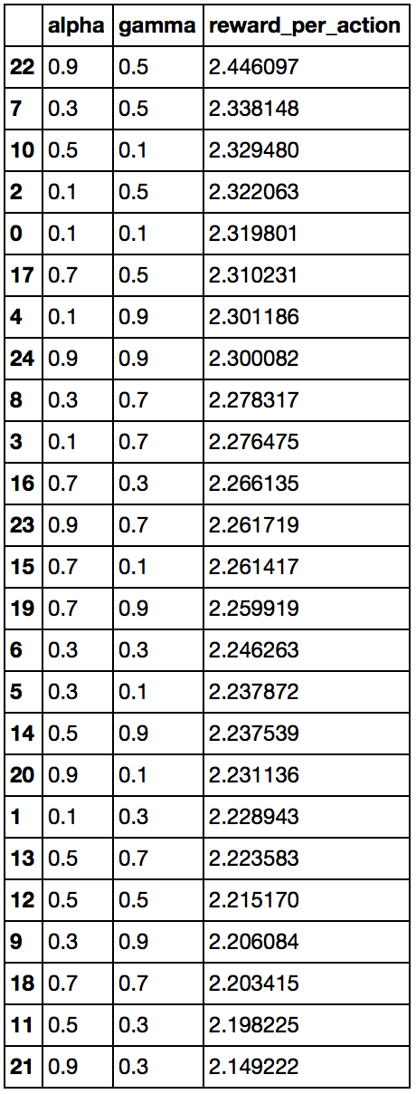
So I actually made my own “grid-search” by testing different learning rate and discount factor values, and calculating the $average\ reward\ /\ total\ moves$ metric for each combination. I set the possible values for the learning rate and alpha as follows: $[0.1, 0.3, 0.5, 0.7, 0.9]$. Thus, there are $25$ combinations total. First, I ran the $100$ trials for each $25$ combination, and got the following result. It seems that the best learning rate to discount factor pair is when learning rate is $0.9$ and discount factor is $0.5$, while the worst one is when the learning rate is $0.9$ but the discount factor $0.3$, resulting in RPM of $2.446 $ and $2.149$ respectively.

Results of Running Experiments with Different Learning Rate and Discount Factor Values

However, this was only $1$ run of $100$ trials for each of the combination. I think that there is a lot of variability and inherent randomness in the placement of dummy cars relative to the learning agent, and also there is randomness in the placement of the learning agent relative to the destination. To be more confident about our results, for each combination of parameters, we could have run many more experiments of $100$ trials and then do Analysis of Variance to see if at least of the groups RPM data varies significantly from the others. However, that would have taken a lot of time, considering that $1$ run of $100$ trials takes almost $2$ minutes. So if I decided to do ANOVA, I would have ran each combination maybe at least $10$ times. That would have taken a long time:

$25$ combinations * $10$ experiments / combination * $2$ minutes / experiment * $1$ hour / $60$ minutes = $8.33$ hours

The shortcut I did instead, was to just focus on the pairs that had the maximum and minimum RPM, ran $15$ experiments for each pair, and then took a difference of two means for each group. I wanted to see whether or not these settings give significantly different results. Given that the original run of $100$ trials for alpha=$0.9$, gamma=$0.3$ resulted in $2.149222$ RPA and alpha=$0.9$, gamma=$0.5$ in $2.446097$ RPA, which is slightly higher than the latter, I expected the average of the set of rewards per action for alpha=$0.9$ and gamma=$0.5$ to be higher than the set for alpha=$0.9$ and gamma=$0.3$, but that does not seem to be the case. This suggests that changing the alpha and gamma values, considering the current the “best action” decision criteria, might be of little consequence.

To further investigate whether or not changing the pair of parameter settings (learning rate, discount factor) from $(0.9, 0.5)$ to $(0.9, 0.3)$ actually makes a difference on RPA, I calculated the p-value with the following, using shuffling:

Calculate the original group means, and subtract them.
Set counter to $0$
Run $10,000$ experiments of the following
- Assume that the null hypothesis is true by shuffling the data between the two groups.
- Calculate the group means and subtract them.
- See if the original difference between two means has been surpassed by that of the shuffled one.
- if so increase counter by 1
P-value is then the counter divided by $10,000$.

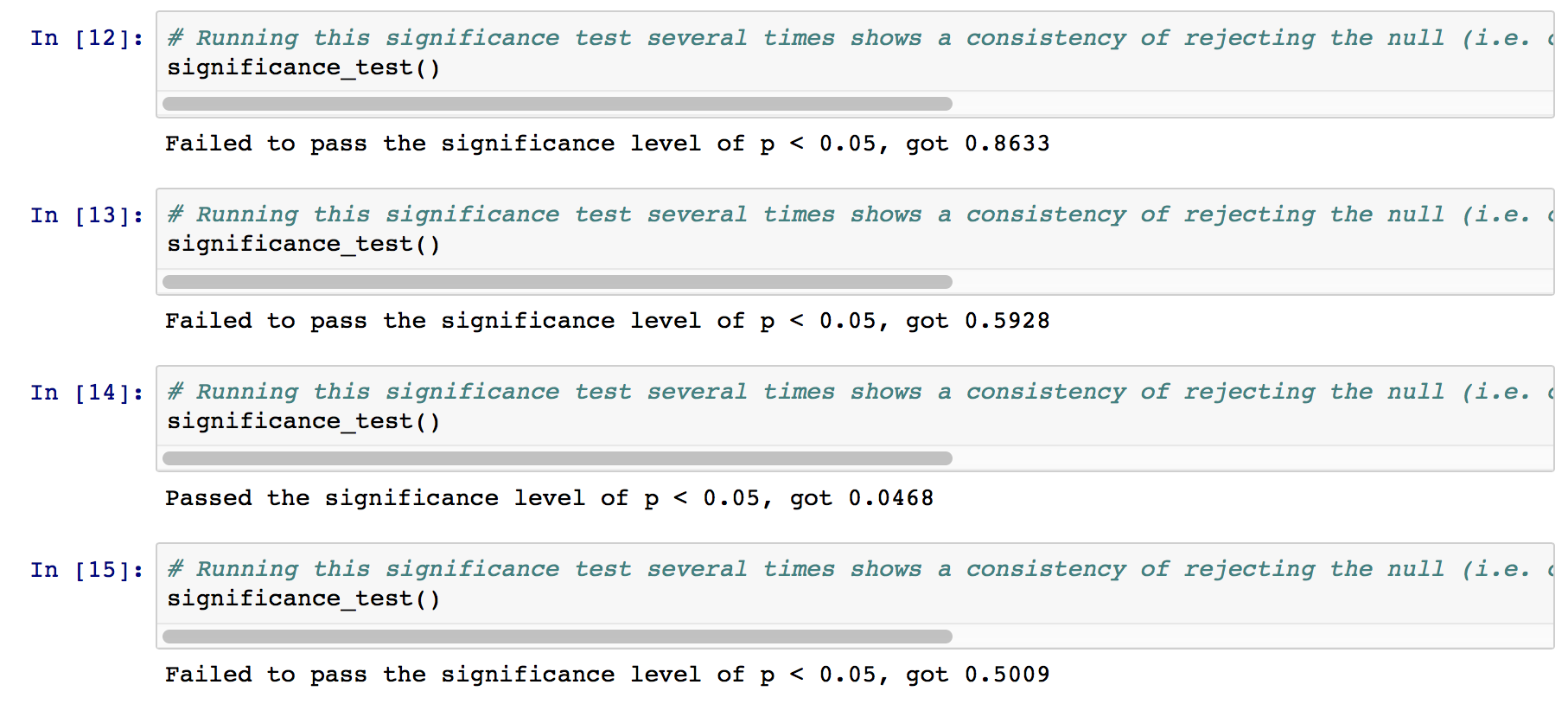
Several runs of the p-value calculation strongly suggest that we should fail to reject the null hypothesis (i.e. the difference of two means between the two groups of different parameters might just really be due to chance). In some runs, p-value does go under $0.05$, but most of the time, it doesn’t. In the cases when it does not, it sometimes reaches really high values. See below:

Does your agent get close to finding an optimal policy, i.e. reach the destination in the minimum possible time, and not incur any penalties?

My agent is definitely close to having the optimal policy. In 100 iterations, it consistently reaches the destination, and minimally incurs penalties (especially in the beginning). After $100$ iterations, it seems to consistently take correct actions. One thing I would add is that the “learning” could probably be accelerated by creating more dummy agents (i.e. it would speed up convergence for states that were happening less often by making those events happen more frequently). By increasing the number of dummy agents, the car would probably interact more with them, and would accumulate penalties to avoid earlier than later. This would then translate to less “training time”, and would be a nice enhancement.